• These notes were prepared while studying for technical interviews (e.g., Snap Inc., Krafton, etc.).
• Each entry contains a concise English summary, key math expressions, and excerpts from my original handwritten/typed study notes.

These notes cover the family of latent-variable and adversarial generative models — how to compress data into representations, how to make those representations probabilistic, and how to train generators by competing against a discriminator.

AutoEncoder

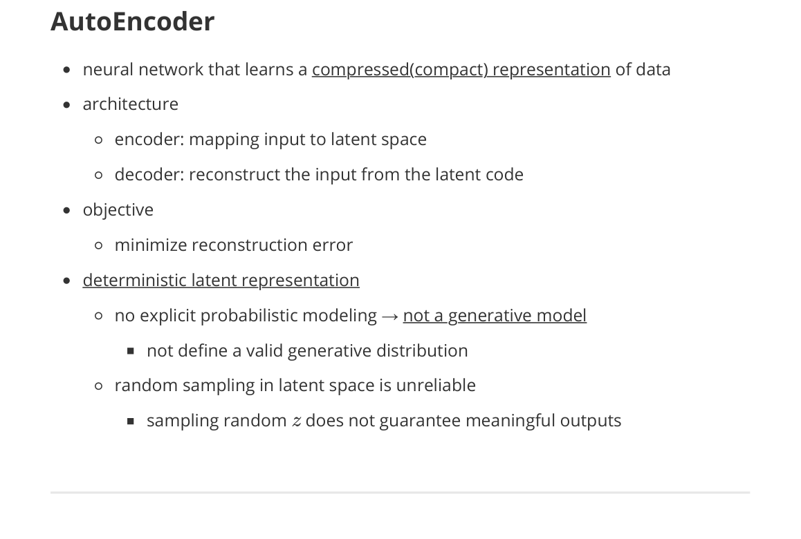
• neural network that learns a compressed (compact) representation of data

Architecture

• Encoder: maps input to latent space
• Decoder: reconstructs the input from the latent code

Objective

• minimize reconstruction error

Deterministic latent representation

• no explicit probabilistic modeling → not a generative model
  • does not define a valid generative distribution
• random sampling in latent space is unreliable
  • sampling random $z$ does not guarantee meaningful outputs

Variational AutoEncoder (VAE)

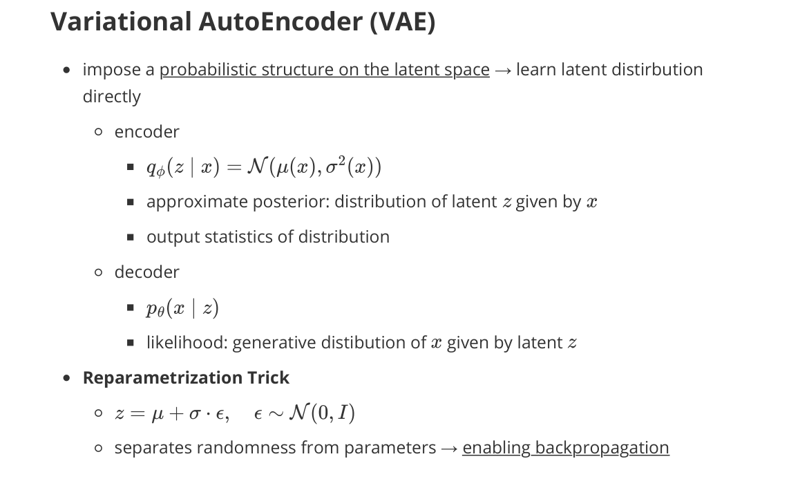
• imposes a probabilistic structure on the latent space → learns a latent distribution directly

Encoder

• $q_\phi(z \mid x) = \mathcal{N}(\mu_\phi(x), \sigma_\phi^2(x))$
• approximate posterior: distribution of latent $z$ given by $x$
• outputs statistics of the distribution

Decoder

• $p_\theta(x \mid z)$
• likelihood: generative distribution of $x$ given by latent $z$

Reparameterization Trick

• separates randomness from parameters → enables backpropagation
• $z = \mu_\phi(x) + \sigma_\phi(x) \odot \epsilon$, $\epsilon \sim \mathcal{N}(0, I)$

Objective

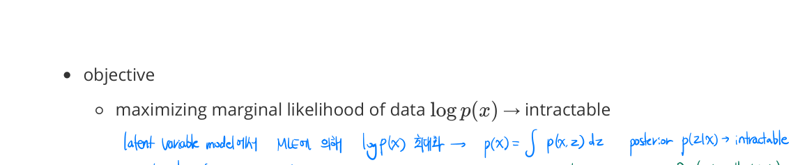
• maximize the marginal log-likelihood of the data: $\log p(x) = \log \int p_\theta(x, z) \, dz$
• intractable in general — the posterior $p(z \mid x)$ is intractable
• → motivates the ELBO (variational lower bound)

ELBO (Evidence Lower BOund)

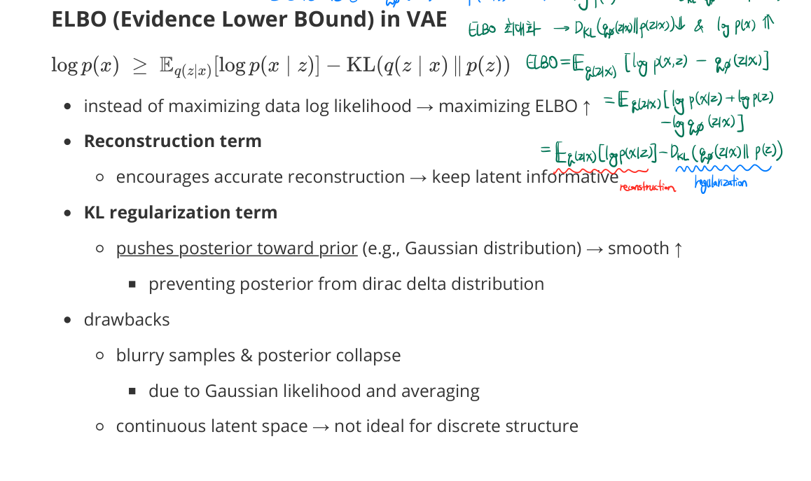
• direct maximization of $\log p(x) = \log \int p_\theta(x, z) \, dz$ is intractable

• maximize ELBO instead:

  \[\log p_\theta(x) \geq \mathbb{E}_{q_\phi(z \mid x)}[\log p_\theta(x \mid z)] - \text{KL}\!\left( q_\phi(z \mid x) \,\big\|\, p(z) \right)\]
• Reconstruction term
  • encourages accurate reconstruction → keep latent informative
• KL regularization term
  • pushes posterior toward prior (e.g., Gaussian distribution) → smooth ↑
    • preventing posterior from Dirac delta distribution

Drawbacks

• blurry samples & posterior collapse
  • due to Gaussian likelihood and averaging
• continuous latent space → not ideal for discrete structure

Vector-Quantized VAE (VQ-VAE)

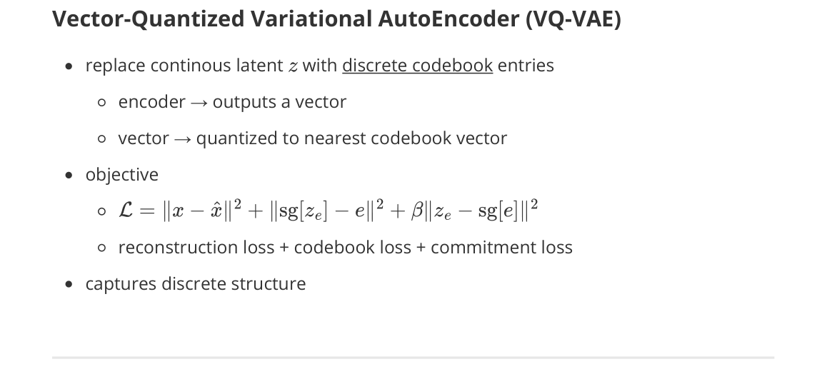
• replace continuous latent $z$ with discrete codebook entries
  • encoder → outputs a vector
  • vector → quantized to nearest codebook vector
• objective
  • $\mathcal{L} = |x - \hat{x}|^2 + |\operatorname{sg}[z_e] - e|^2 + \beta |z_e - \operatorname{sg}[e]|^2$
  • reconstruction loss + codebook loss + commitment loss
• captures discrete structure

Generative Model

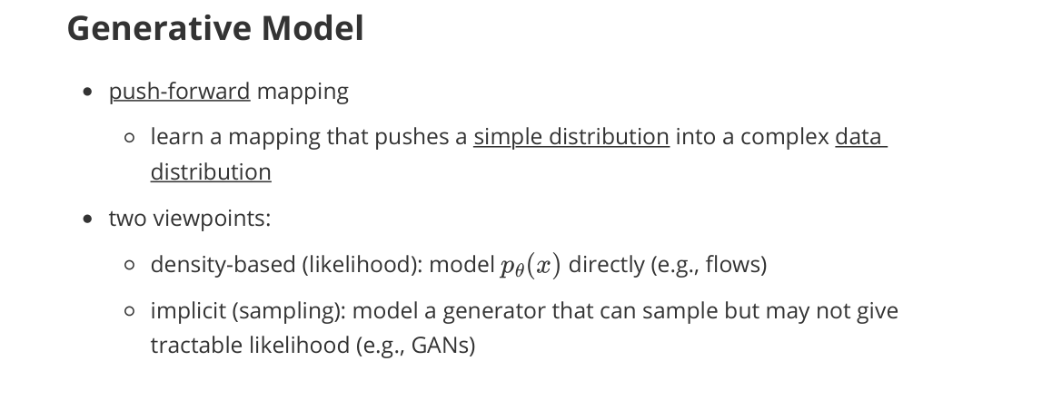
• Push-forward mapping
  • learn a mapping that pushes a simple distribution into a complex data distribution
• two viewpoints
  • density-based (likelihood): model $p_\theta(x)$ directly (e.g., flows)
  • implicit (sampling): model a generator that can sample but may not give tractable likelihood (e.g., GANs)

Evaluation Metrics

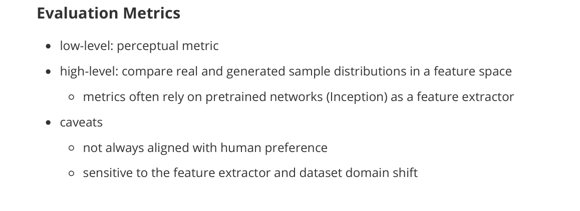
• low-level: perceptual metric
• high-level: compare real and generated sample distributions in a feature space
  • metrics often rely on pretrained networks (Inception) as a feature extractor
• caveats
  • not always aligned with human preference
  • sensitive to the feature extractor and dataset domain shift

Peak Signal-to-Noise Ratio (PSNR)

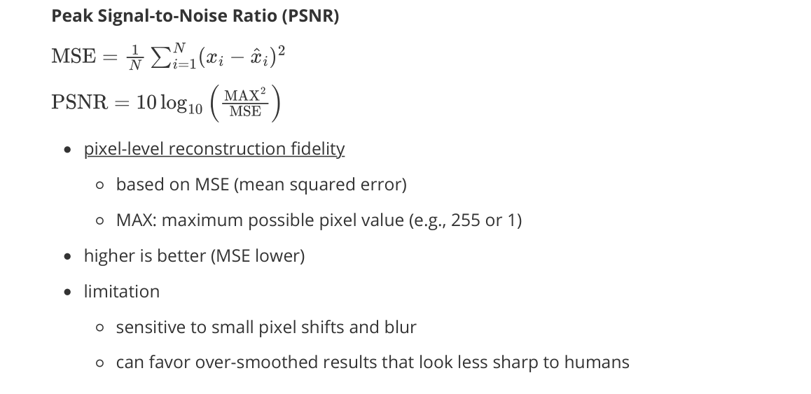
• pixel-level reconstruction fidelity
  • based on MSE (mean squared error)
  • MAX: maximum possible pixel value (e.g., 255 or 1)
• higher is better (MSE lower)
• limitation
  • sensitive to small pixel shifts and blur
  • can favor over-smoothed results that look less sharp to humans

Structural Similarity Index (SSIM)

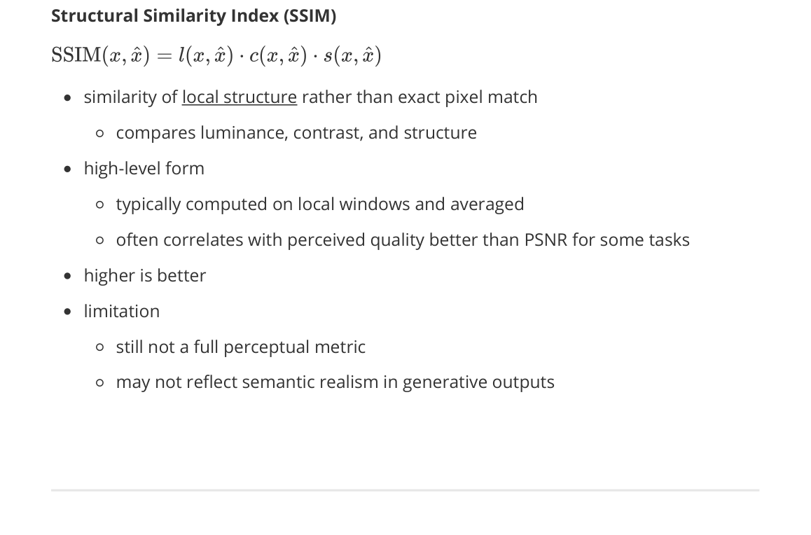
• similarity of local structure rather than exact pixel match
  • compares luminance, contrast, and structure
• high-level form
  • typically computed on local windows and averaged
  • often correlates with perceived quality better than PSNR for some tasks
• higher is better
• limitation
  • still not a full perceptual metric
  • may not reflect semantic realism in generative outputs

Fréchet Inception Distance (FID)

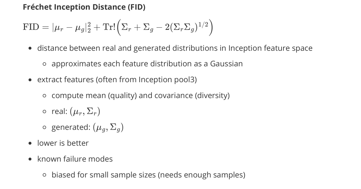
• distance between real and generated distributions in Inception feature space
  • approximates each feature distribution as a Gaussian
• extract features (often from Inception pool3)
  • compute mean (quality) and covariance (diversity)
  • real: $(\mu_r, \Sigma_r)$
  • generated: $(\mu_g, \Sigma_g)$
• lower is better
• known failure modes
  • biased for small sample sizes (needs enough samples)
  • can be gamed if feature extractor is inappropriate

Inception Score

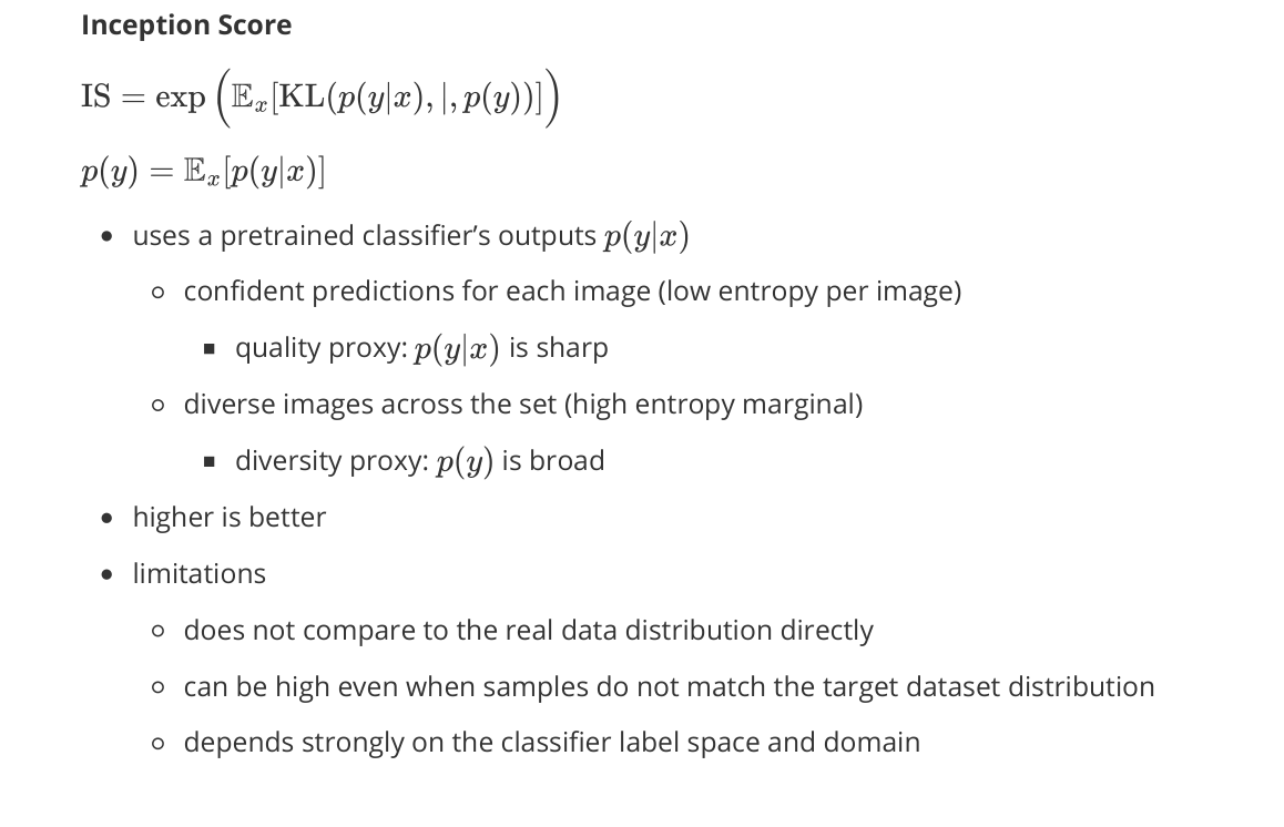
• uses a pretrained classifier’s outputs $p(y \mid x)$
  • confident predictions for each image (low entropy per image)
    • quality proxy: $p(y \mid x)$ is sharp
  • diverse images across the set (high entropy marginal)
    • diversity proxy: $p(y)$ is broad
• higher is better
• limitations
  • does not compare to the real data distribution directly
  • can be high even when samples do not match the target dataset distribution
  • depends strongly on the classifier label space and domain

Learned Perceptual Image Patch Similarity (LPIPS)

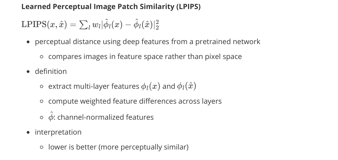
• perceptual distance using deep features from a pretrained network
  • compares images in feature space rather than pixel space
• definition
  • extract multi-layer features $\phi_l(x)$ and $\phi_l(\hat{x})$
  • compute weighted feature differences across layers
  • $\hat{\phi}$: channel-normalized features
• interpretation
  • lower is better (more perceptually similar)
  • commonly used for image-to-image translation, restoration, diffusion reconstruction quality
• limitation
  • depends on the backbone and training domain
  • not a distribution metric (unlike FID) — it’s a pairwise similarity metric

Generative Adversarial Network (GAN)

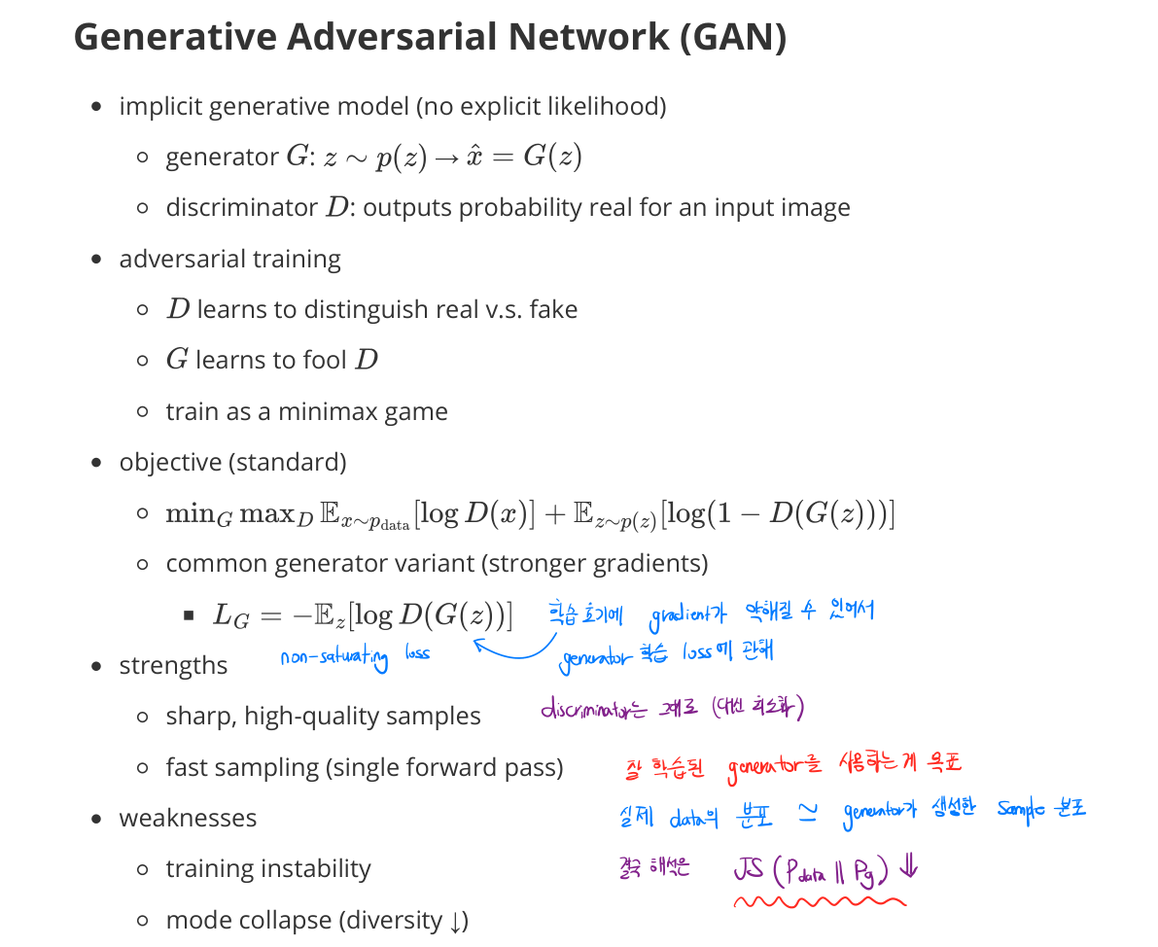
• implicit generative model (no explicit likelihood)
  • generator $G$: $z \sim p(z) \to \hat{x} = G(z)$
  • discriminator $D$: outputs probability real for an input image

Adversarial training

• $D$ learns to distinguish real v.s. fake
• $G$ learns to fool $D$
• train as a minimax game

Objective (standard)

• \[\min_G \max_D \; \mathbb{E}_{x \sim p_{\text{data}}}[\log D(x)] + \mathbb{E}_{z \sim p(z)}[\log(1 - D(G(z)))]\]
• common generator variant (stronger gradients early in training)
  • $\mathcal{L}_G = -\mathbb{E}_z[\log D(G(z))]$ — non-saturating loss

Strengths

• sharp, high-quality samples
• fast sampling (single forward pass)

Weaknesses

• training instability
• mode collapse (diversity ↓)

Wasserstein GAN (WGAN)

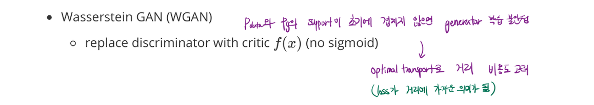
• replace discriminator with a critic $D$ (no sigmoid)
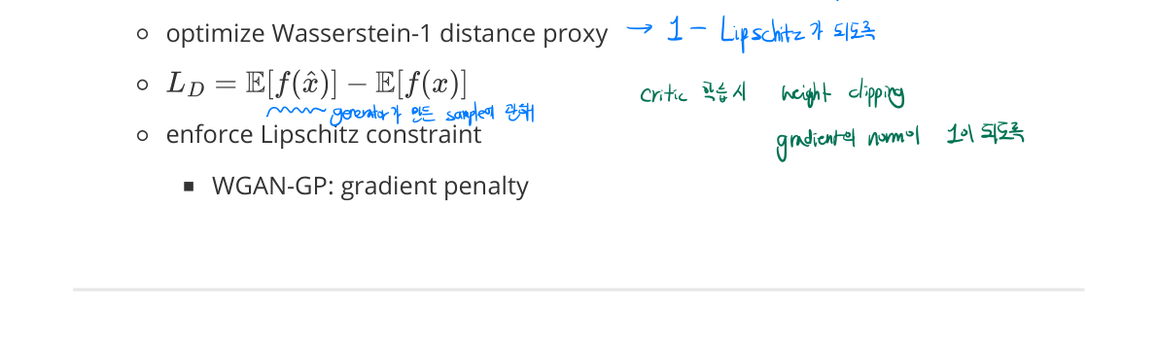
  • optimize Wasserstein-1 distance proxy
  • critic loss: $\mathcal{L}_D = \mathbb{E}[f(\hat{x})] - \mathbb{E}[f(x)]$
  • enforce Lipschitz constraint (weight clipping or gradient penalty)
    • WGAN-GP: gradient penalty on the critic
• mitigates issues where the supports of $p_{\text{data}}$ and $p_g$ don’t overlap → unstable generator training