• These notes were prepared while studying for technical interviews (e.g., Snap Inc., Krafton, etc.).
• Each entry contains a concise English summary, key math expressions, and excerpts from my original handwritten/typed study notes.

These notes cover the foundations of discriminative classification and the information-theoretic objectives that drive most learning losses.

Support Vector Machine (SVM)

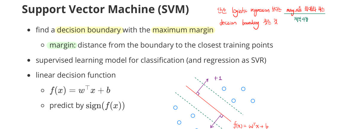
• find a decision boundary with the maximum margin
  • margin: distance from the boundary to the closest training points
• supervised learning model for classification (and regression as SVR)
• linear decision function
  • $f(x) = w^\top x + b$
  • predict by $\operatorname{sign}(f(x))$

Maximum-Margin (Hard Margin)

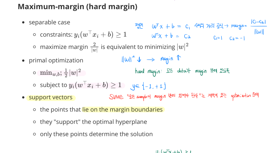
• separable case
  • constraints: $y_i(w^\top x_i + b) \geq 1$
  • maximize margin $\frac{2}{|w|}$ is equivalent to minimizing $\frac{1}{2}|w|^2$

• primal optimization:

  \[\min_{w,b} \tfrac{1}{2}\|w\|^2 \quad \text{s.t.} \quad y_i(w^\top x_i + b) \geq 1\]
• Support vectors
  • the points that lie on the margin boundaries
  • they “support” the optimal hyperplane
  • only these points determine the solution

Soft Margin (Non-Separable)

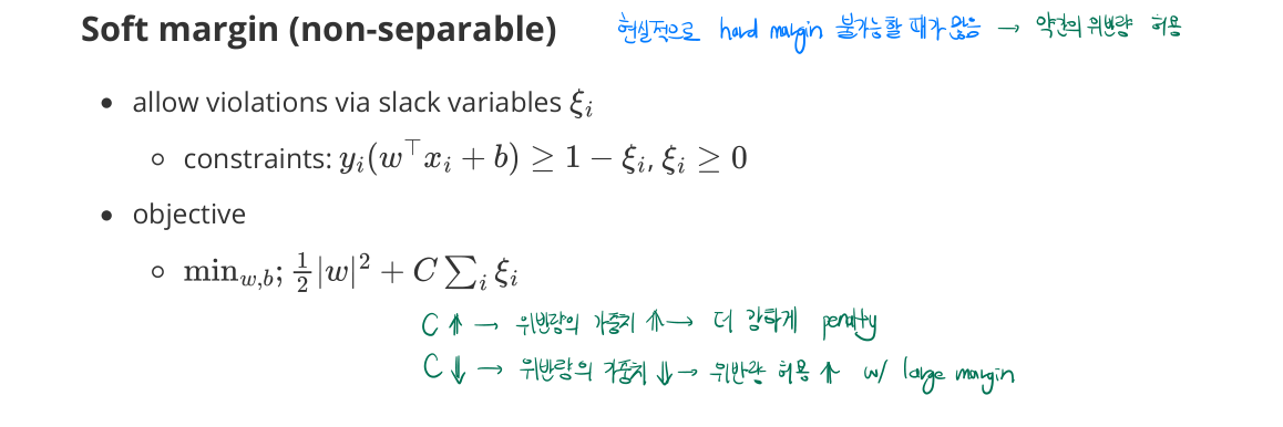
• allow violations via slack variables $\xi_i \geq 0$
  • constraints: $y_i(w^\top x_i + b) \geq 1 - \xi_i$

• objective:

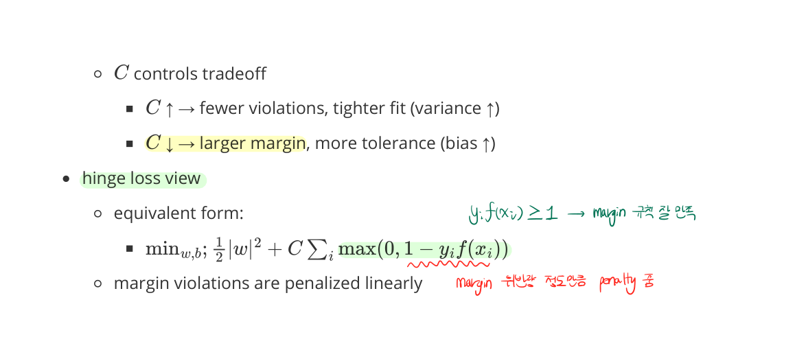
  \[\min_{w,b,\xi} \tfrac{1}{2}\|w\|^2 + C \sum_i \xi_i\]
• $C$ controls tradeoff
  • $C \uparrow$ → fewer violations, tighter fit (variance ↑)
  • $C \downarrow$ → larger margin, more tolerance (bias ↑)

• hinge loss view:

  \[\min_{w,b} \tfrac{1}{2}\|w\|^2 + C \sum_i \max(0, 1 - y_i f(x_i))\]
• margin violations are penalized linearly

Kernel Trick

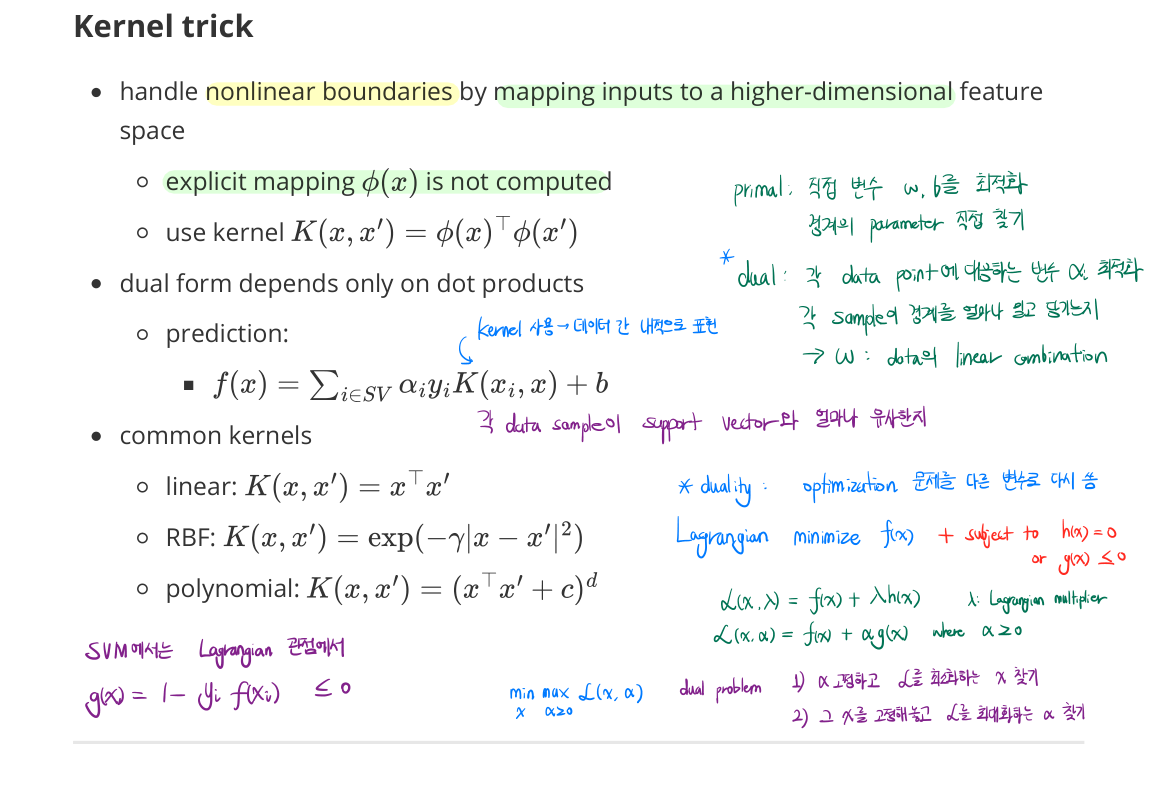
• handle nonlinear boundaries by mapping inputs to a higher-dimensional feature space
  • explicit mapping $\phi(x)$ is not computed
  • use kernel $K(x, x’) = \phi(x)^\top \phi(x’)$
• dual form depends only on dot products
  • prediction:
    • $f(x) = \sum_{i \in \text{SV}} \alpha_i y_i K(x_i, x) + b$
• common kernels
  • linear: $K(x, x’) = x^\top x’$
  • RBF: $K(x, x’) = \exp(-\gamma |x - x’|^2)$
  • polynomial: $K(x, x’) = (x^\top x’ + c)^d$

Logit & Softmax

Logit

• logarithm of the odds of the event
  • raw & unnormalized scores output by the model
  • pre-softmax outputs whose differences correspond to log-odds between classes
• interpreted as evidence for each class

Softmax

• convert logits into a probability distribution
  • output is positive and sums to 1
  • preserve relative differences between logits
• smooth and differentiable
  • compatible with likelihood-based objectives
• $e^{z}$ grows extremely fast
  • if some logit $z$ is large, $e^{z}$ can exceed floating-point range → overflow (inf)

Log-Sum-Exp Trick

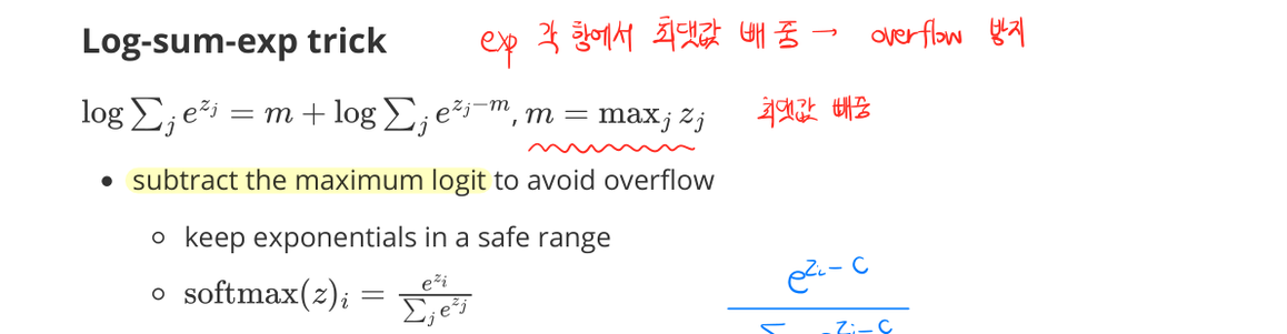
• subtract the maximum logit to avoid overflow
  • keeps exponentials in a safe range

Gumbel Softmax

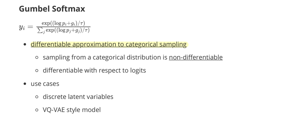
• differentiable approximation to categorical sampling
  • sampling from a categorical distribution is non-differentiable
  • differentiable with respect to logits
• use cases
  • discrete latent variables
  • VQ-VAE style models

Entropy

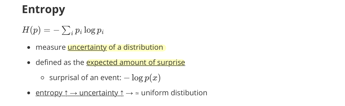
• measure uncertainty of a distribution
• defined as the expected amount of surprise
  • surprisal of an event: $-\log p(x)$
• entropy ↑ → uncertainty ↑ → ≃ uniform distribution
• entropy ↓ → more confident or peaked distribution → ≃ deterministic distribution

Cross-Entropy

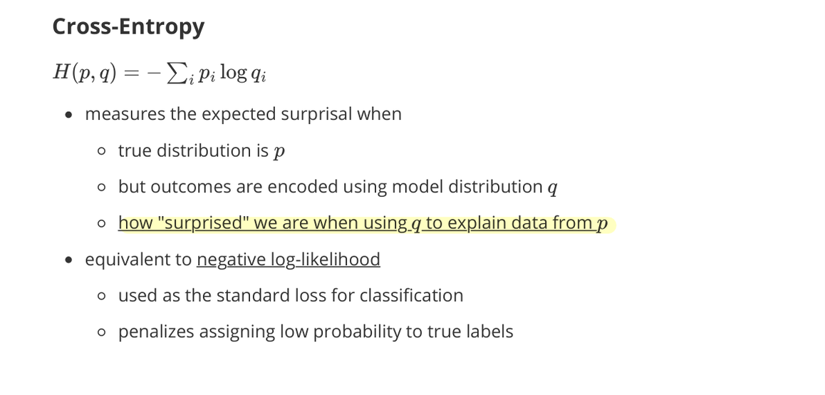
• measures the expected surprisal when
  • true distribution is $p$
  • but outcomes are encoded using model distribution $q$
  • how “surprised” we are when using $q$ to explain data from $p$
• equivalent to negative log-likelihood
  • used as the standard loss for classification
  • penalizes assigning low probability to true labels

KL Divergence

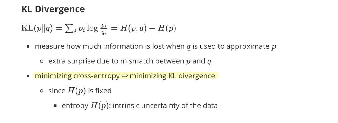
• measure how much information is lost when $q$ is used to approximate $p$
  • extra surprise due to mismatch between $p$ and $q$
• minimizing cross-entropy ⇔ minimizing KL divergence
  • since $H(p)$ is fixed
    • entropy $H(p)$: intrinsic uncertainty of the data