• These notes were prepared while studying for technical interviews (e.g., Snap Inc., Krafton, etc.).
• Each entry contains a concise English summary, key math expressions, and excerpts from my original handwritten/typed study notes.

These notes cover the convolutional building blocks that power modern computer-vision architectures, and the residual learning idea that made training very deep networks possible.

Convolutional Neural Networks (CNN)

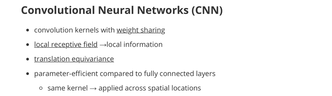
• convolution kernels with weight sharing
• local receptive field → local information
• translation equivariance
• parameter-efficient compared to fully connected layers
  • same kernel → applied across spatial locations

Downsampling

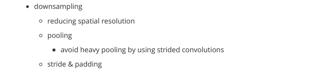
• reducing spatial resolution
• pooling
  • avoid heavy pooling by using strided convolutions
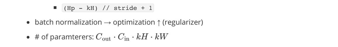
• stride & padding: output size = $(H_{\text{in}} - k_H) / s + 1$
• batch normalization → optimization ↑ (also acts as a regularizer)

Convolution Variants

Standard convolution

• parameters: $C_{\text{in}} \cdot C_{\text{out}} \cdot k_H \cdot k_W$

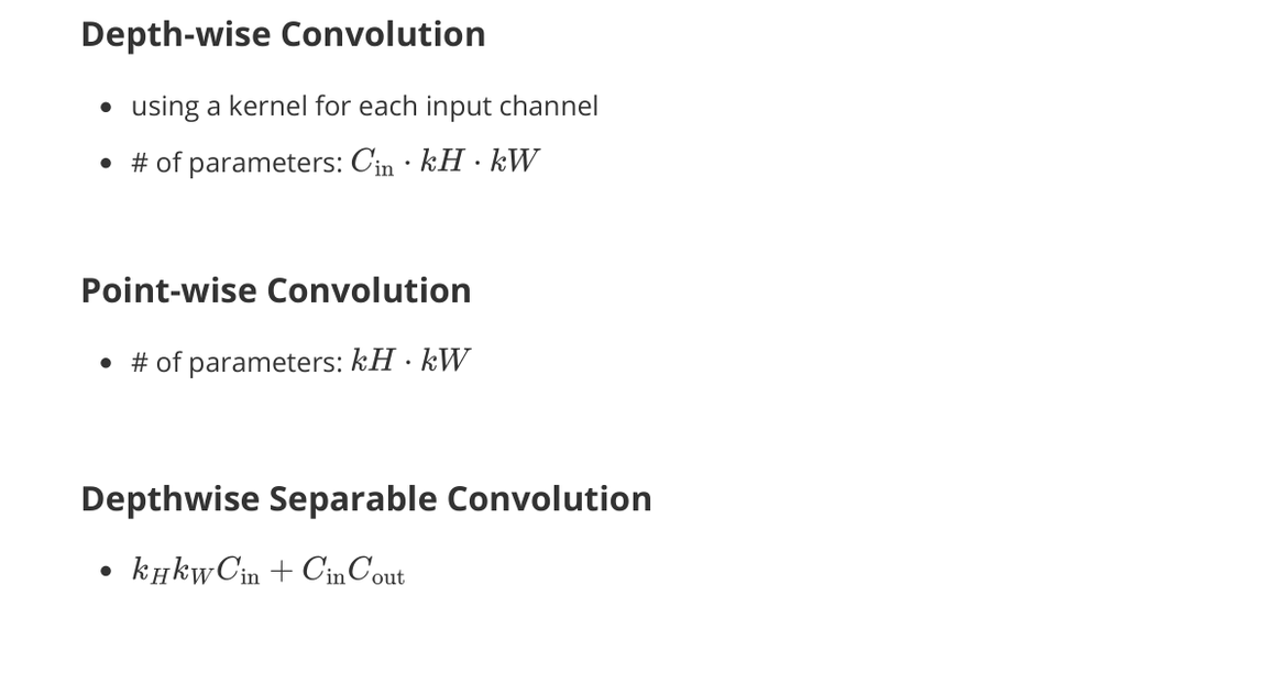
Depthwise Convolution

• using a kernel for each input channel
• parameters: $C_{\text{in}} \cdot k_H \cdot k_W$

Pointwise Convolution

• $1 \times 1$ convolution
• parameters: $C_{\text{in}} \cdot C_{\text{out}}$

Depthwise Separable Convolution

• depthwise + pointwise → mixing spatial and channel-wise computations cheaply
• parameters: $k_H k_W C_{\text{in}} + C_{\text{in}} C_{\text{out}}$

Adaptive Average Pooling

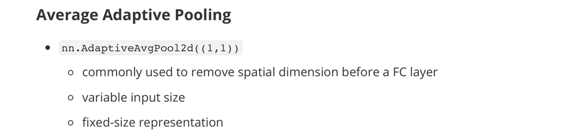
• nn.AdaptiveAvgPool2d((1,1))
  • commonly used to remove spatial dimension before a FC layer
  • variable input size
  • fixed-size representation

ResNet

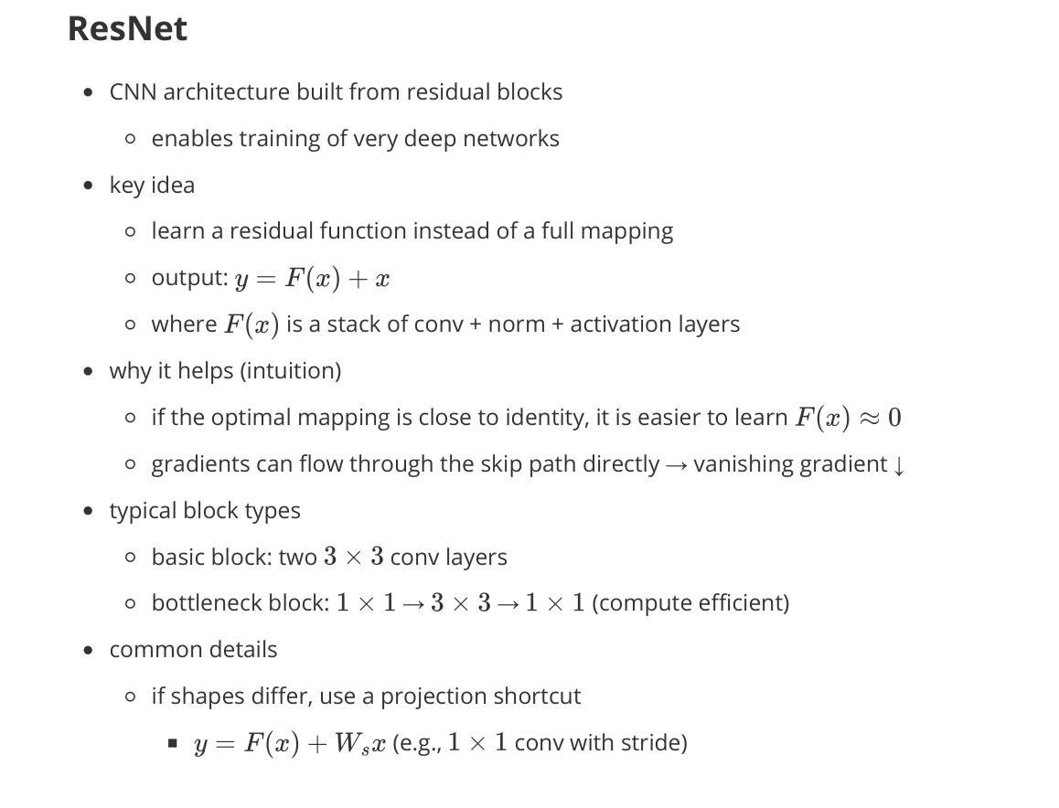
• CNN architecture built from residual blocks
  • enables training of very deep networks

Key idea

• learn a residual function instead of a full mapping
• output: $y = F(x) + x$
• where $F(x)$ is a stack of conv + norm + activation layers

Why it helps (intuition)

• if the optimal mapping is close to identity, it is easier to learn $F(x) \approx 0$
• gradients can flow through the skip path directly → vanishing gradient ↓

Typical block types

• Basic block: two $3 \times 3$ conv layers
• Bottleneck block: $1 \times 1$ → $3 \times 3$ → $1 \times 1$ (compute-efficient)

Common details

• if shapes differ, use a projection shortcut
  • $y = F(x) + W_s x$ (e.g., $1 \times 1$ conv with stride)

Residual Connection

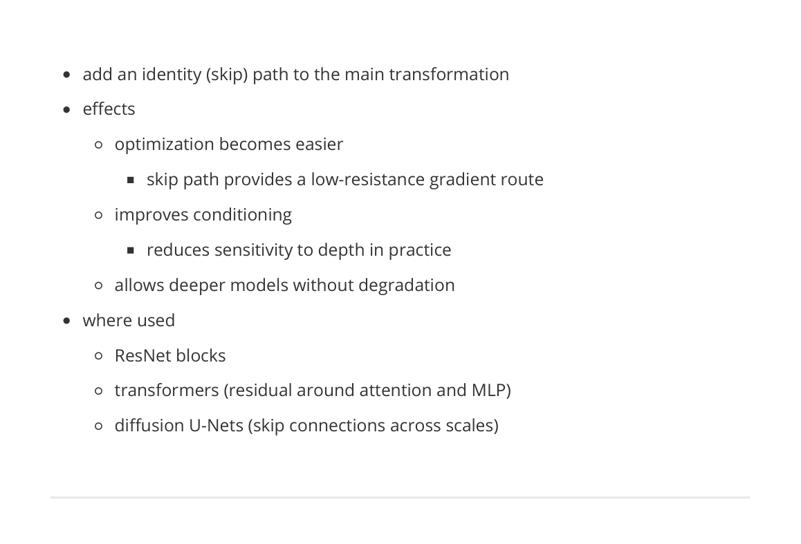
• add an identity (skip) path to the main transformation

Effects

• optimization becomes easier
  • skip path provides a low-resistance gradient route
• improves conditioning
  • reduces sensitivity to depth in practice
• allows deeper models without degradation

Where used

• ResNet blocks
• Transformers (residual around attention and MLP)
• Diffusion U-Nets (skip connections across scales)