• These notes were prepared while studying for technical interviews (e.g., Snap Inc., Krafton, etc.).
• Each entry contains a concise English summary, key math expressions, and excerpts from my original handwritten/typed study notes.

These notes cover the modern continuous-time generative-modeling family — denoising diffusion, the score-based SDE viewpoint, classifier-free guidance, and the flow-matching reformulation that unifies them. The handwritten pages at the end derive the SDE / score-model / sampler / solver mechanics in detail.

Denoising Diffusion

• decomposing the mapping into a sequence of small, incremental transformations
  • from a simple distribution (e.g., Gaussian noise)
  • to a complex data distribution
• learn to reverse a gradual noising process
  • instead of directly learning a single complex mapping from noise to data

DDPM (Denoising Diffusion Probabilistic Models)

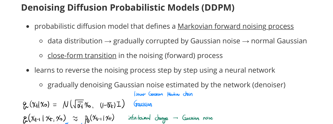
• probabilistic diffusion model that defines a Markovian forward noising process
  • data distribution → gradually corrupted by Gaussian noise → standard Gaussian
  • closed-form transition in the noising (forward) process

• learns to reverse the noising process step by step using a neural network
  • gradually denoising Gaussian noise estimated by the network (denoiser)
  • true posterior is approximated by the learned reverse step

DDIM (Denoising Diffusion Implicit Models)

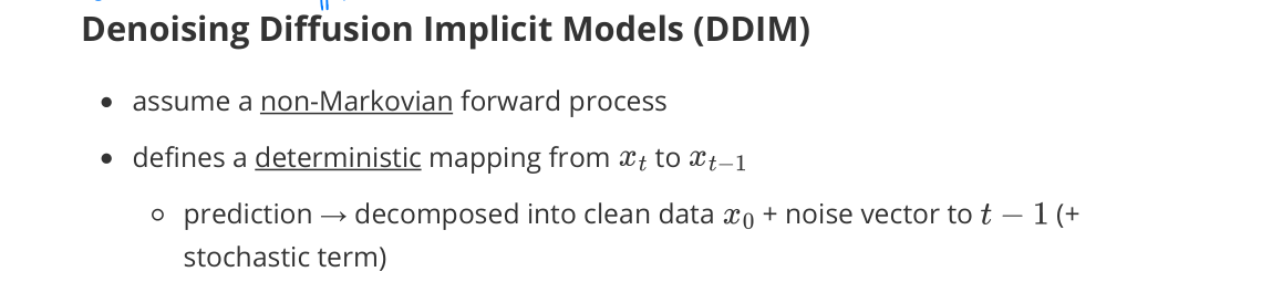
• assume a non-Markovian forward process
• defines a deterministic mapping from $x_t$ to $x_{t-1}$
  • prediction → decomposed into clean data $x_0$ + noise vector to $t-1$ (+ stochastic term)
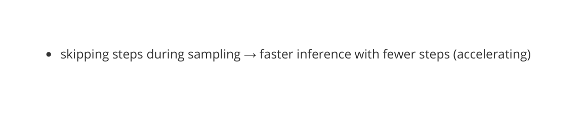
• skipping steps during sampling → faster inference with fewer steps (accelerating)

Classifier-Free Guidance (CFG)

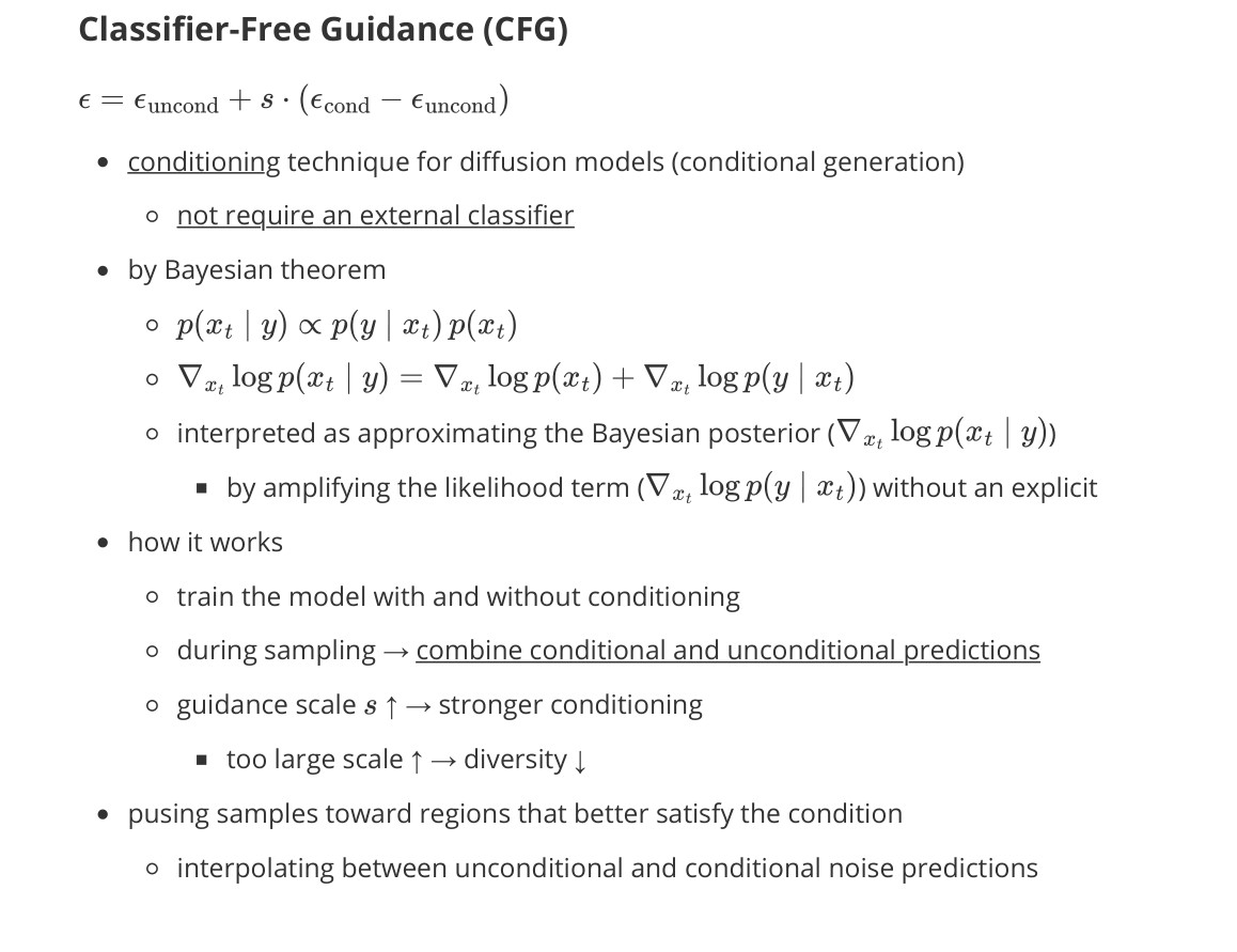
• conditioning technique for diffusion models (conditional generation)
  • does not require an external classifier
• by Bayes’ theorem
  • $p(x_t \mid y) \propto p(y \mid x_t)\, p(x_t)$
  • $\nabla_{x_t} \log p(x_t \mid y) = \nabla_{x_t} \log p(x_t) + \nabla_{x_t} \log p(y \mid x_t)$
  • interpreted as approximating the Bayesian posterior $\nabla_{x_t} \log p(x_t \mid y)$
    • by amplifying the likelihood term $\nabla_{x_t} \log p(y \mid x_t)$ without an explicit classifier

How it works

• train the model with and without conditioning

• during sampling → combine conditional and unconditional predictions:

  \[\tilde{\epsilon}_\theta(x_t, c) = (1 + w) \epsilon_\theta(x_t, c) - w \epsilon_\theta(x_t, \varnothing)\]
• guidance scale $w \uparrow$ → stronger conditioning
  • too large $w$ → diversity ↓
• pushes samples toward regions that better satisfy the condition
  • interpolates between unconditional and conditional noise predictions

Score Function

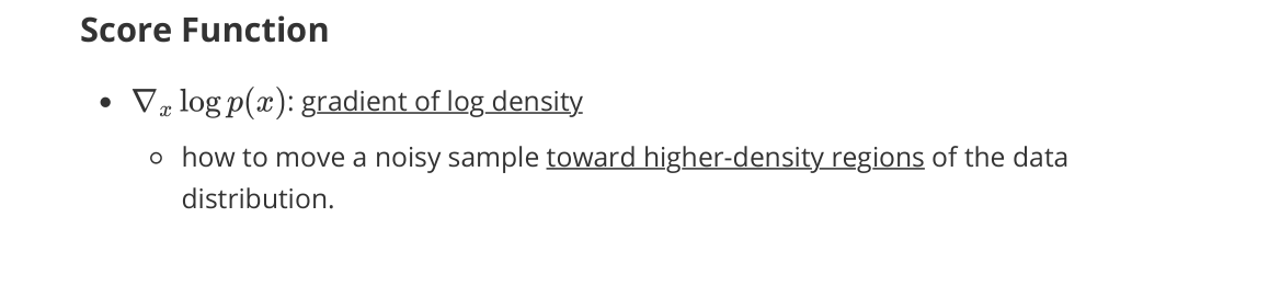
• $\nabla_x \log p(x)$: gradient of log density
  • describes how to move a noisy sample toward higher-density regions of the data distribution

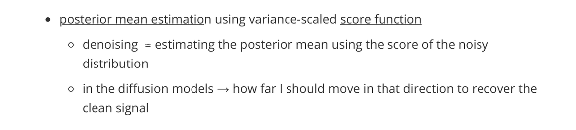
Tweedie’s Formula

• posterior mean estimation using variance-scaled score function:

  \[\mathbb{E}[x_0 \mid x_t] = \frac{x_t + \sigma_t^2 \nabla_{x_t} \log p_t(x_t)}{\sqrt{\bar{\alpha}_t}}\]
• denoising ≃ estimating the posterior mean using the score of the noisy distribution
• in diffusion models: how far to move in the score direction to recover the clean signal

Flow Matching

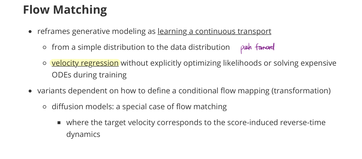
• reframes generative modeling as learning a continuous transport
  • from a simple distribution to the data distribution (push-forward)
  • velocity regression without explicitly optimizing likelihoods or solving expensive ODEs during training
• variants dependent on how to define a conditional flow mapping (transformation)
  • diffusion models: a special case of flow matching
    • where the target velocity corresponds to the score-induced reverse-time dynamics

Normalizing Flow

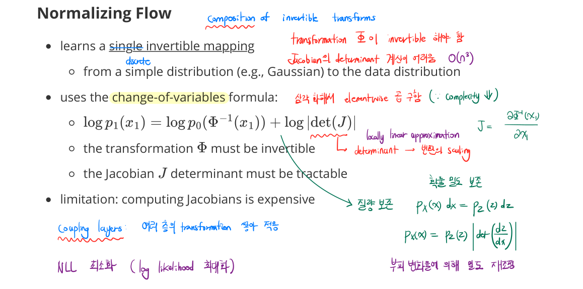
• learns a single invertible mapping
  • from a simple distribution (e.g., Gaussian) to the data distribution
• uses the change-of-variables formula:
  • $\log p_1(x_1) = \log p_0(\Phi^{-1}(x_1)) + \log \lvert \det J \rvert$
  • the transformation $\Phi$ must be invertible
  • the Jacobian $J$ determinant must be tractable
• limitation: computing Jacobians is expensive
  • $O(n^3)$ in general
  • triangularization gives elementwise product → $O(n)$

Continuous Normalizing Flow (CNF)

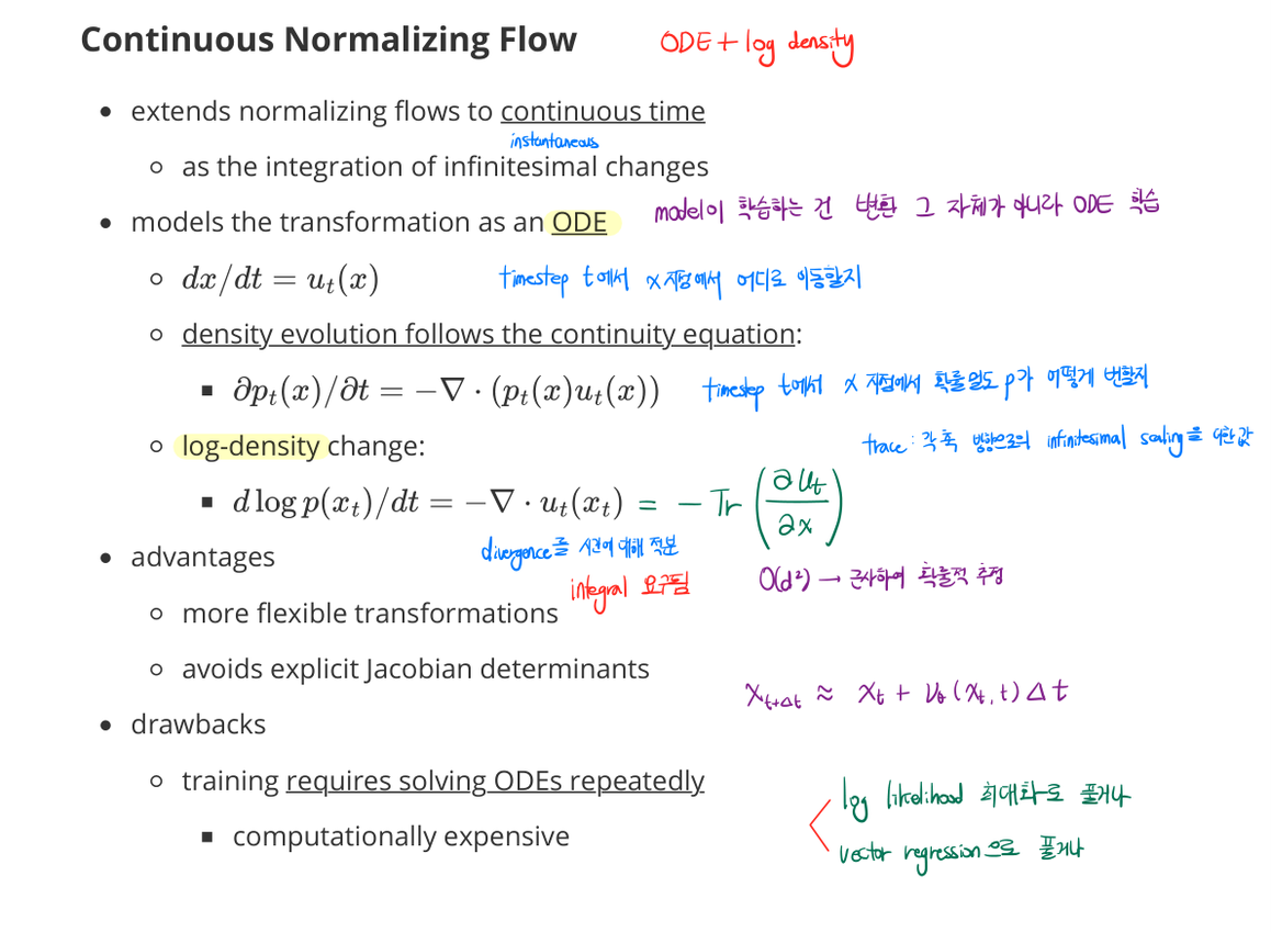
• extends normalizing flows to continuous time
  • as the integration of infinitesimal changes
• models the transformation as an ODE
  • $dx/dt = u_t(x)$
  • density evolution follows the continuity equation:
    • $\partial p_t(x) / \partial t = -\nabla \cdot (p_t(x)\, u_t(x))$
  • log-density change:
    • $d \log p(x_t) / dt = -\nabla \cdot u_t(x_t) = -\operatorname{Tr}!\left(\partial u_t / \partial x\right)$
• advantages
  • more flexible transformations
  • avoids explicit Jacobian determinants
• drawbacks
  • training requires solving ODEs repeatedly
    • computationally expensive

Flow Matching Objective

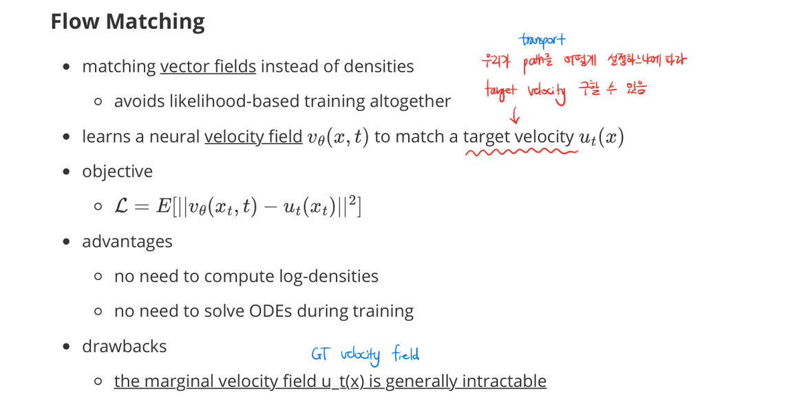
• matching vector fields instead of densities
  • avoids likelihood-based training altogether
• learn a neural velocity field $v_\theta(x, t)$ to match a target velocity $u_t(x)$
  • target velocity is determined by how the transport path is chosen

• advantages: no log-density computation, no ODE solves during training
• drawback: the marginal velocity field $u_t(x)$ is generally intractable

Conditional Flow Matching (CFM)

• learn a conditional velocity field $u_t(x \mid x_0, x_1)$
  • instead of learning a marginal velocity field $u_t(x)$
• samples are paired:
  • $x_0 \sim$ base distribution
  • $x_1 \sim$ data distribution
• learns how to transport $x_0$ to $x_1$ over time
• objective
  • $\mathcal{L} = \mathbb{E}!\left[|v_\theta(x_t, t) - u_t(x_t \mid x_0, x_1)|^2\right]$
  • theoretically grounded by the continuity equation
• benefits
  • simpler target vector field
  • stable training
  • avoids density estimation entirely

Rectified Flow

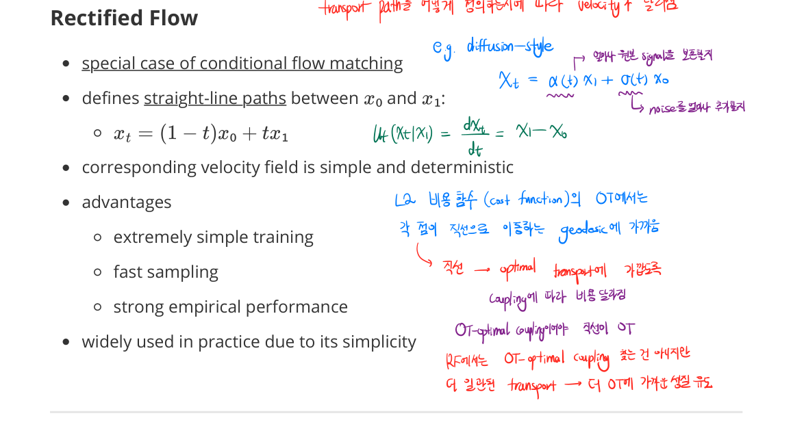
• special case of conditional flow matching
• defines straight-line paths between $x_0$ and $x_1$:
  • $x_t = (1 - t) x_0 + t x_1$
• corresponding velocity field is simple and deterministic: $u_t = x_1 - x_0$
• advantages
  • extremely simple training
  • fast sampling
  • strong empirical performance
• widely used in practice due to its simplicity
• OT-optimal coupling makes the transport closer to a geodesic

Diffusion Transformer (DiT)

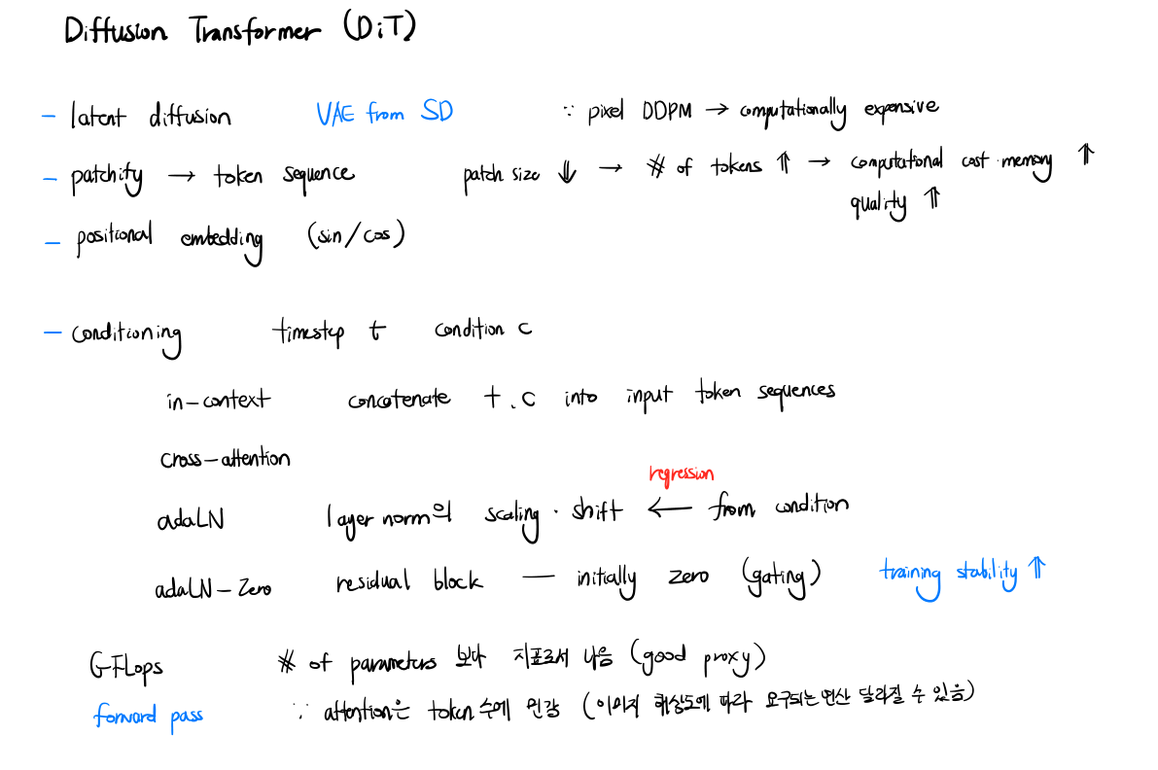
• latent diffusion: VAE from Stable Diffusion, pixel-space DDPM computationally expensive
• Patchify
  • token sequence with patch size $N$
  • smaller patch → more tokens, higher computational cost
  • quality ↑, memory ↑
• Positional embedding: sinusoidal
• Conditioning
  • timestep $t$, condition $c$ (e.g., class label)
  • in-context: concatenate $t, c$ into input token sequence
  • cross-attention: regression
  • adaLN: scaling/shifting of LayerNorm from condition
  • adaLN-Zero: residual block initially zero-gated → training stability
• GFLOPs is a better proxy than parameter count for compute cost
• forward pass attention is sensitive to token count (image resolution affects required compute)

SDE-based Score Model

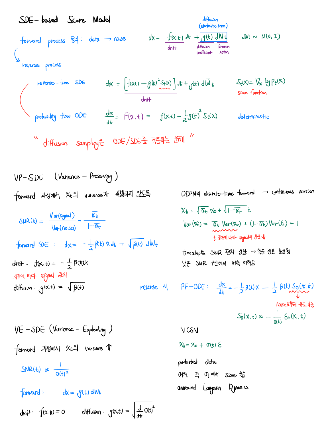
• diffusion as a stochastic process

Forward process

• $f$: drift, $g$: diffusion coefficient, $W_t$: Brownian motion

Reverse-time SDE

• $s_\theta(x, t) = \nabla_x \log p_t(x)$: score function (drift)

Probability Flow ODE

• deterministic; diffusion sampling reduces to integrating ODE / SDE

VP-SDE (Variance Preserving)

• $\text{Var}(x_t)$ does not blow up over time
• DDPM’s discrete-time forward process → continuous version
• $x_t = \sqrt{\bar{\alpha}_t}\, x_0 + \sqrt{1 - \bar{\alpha}_t}\, \epsilon$
• $\text{SNR}(t) = \bar{\alpha}_t / (1 - \bar{\alpha}_t)$
• forward SDE: $dx = -\tfrac{1}{2} \beta(t) x\, dt + \sqrt{\beta(t)}\, dW_t$
• reverse PF-ODE: $\frac{dx}{dt} = -\tfrac{1}{2} \beta(t) x - \tfrac{1}{2} \beta(t) s_\theta(x, t)$

VE-SDE (Variance Exploding)

• NCSN-style: variance grows over time
• $x_t = x_0 + \sigma(t) \epsilon$
• $\text{SNR}(t) \propto 1 / \sigma(t)^2$
• forward: $dx = g(t)\, dW_t$ (drift = 0)
• learns score at many noise levels — annealed Langevin dynamics

Prediction Targets

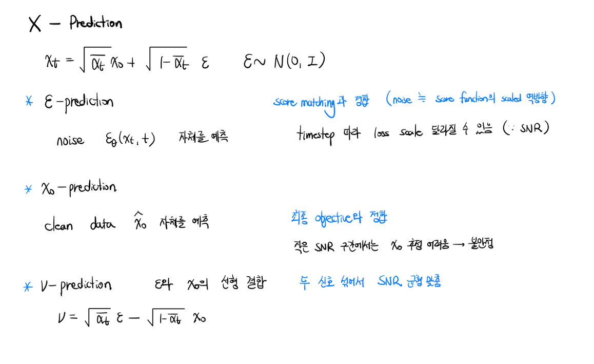
• $\epsilon$-prediction: predict the noise $\epsilon_\theta(x_t, t)$ itself
  • aligns with score matching (noise = scaled negative of the score function)
  • loss scale can vary by timestep (due to SNR)
• $x_0$-prediction: predict the clean data $\hat{x}_0$ directly
  • aligns with the final objective
  • unstable at low SNR (hard to estimate $x_0$)
• v-prediction: linear combination of $\epsilon$ and $x_0$
  • $v = \sqrt{\bar{\alpha}_t}\, \epsilon - \sqrt{1 - \bar{\alpha}_t}\, x_0$
  • mixes the two signals to balance SNR across timesteps

Noise Scheduler

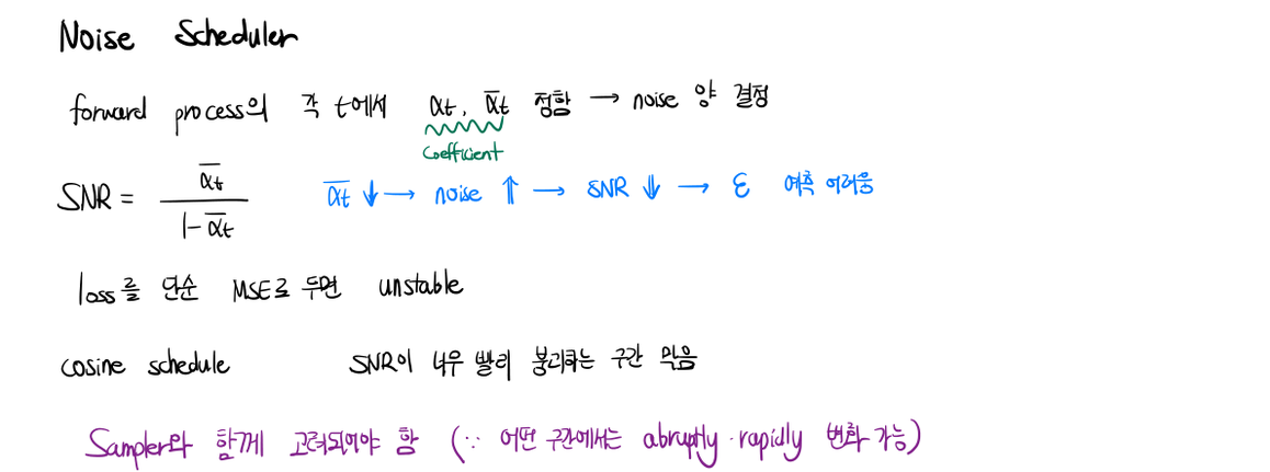
• forward process: choose $\alpha_t, \bar{\alpha}_t$ at each $t$ → determines noise amount
• SNR $= \bar{\alpha}_t / (1 - \bar{\alpha}_t)$
  • $\bar{\alpha}_t \downarrow$ → noise $\uparrow$ → SNR $\downarrow$ → $\epsilon$ prediction harder
• naive MSE loss can be unstable
• cosine schedule: prevents SNR from collapsing too quickly
• must be considered together with the sampler

Sampler & Solver

Sampler

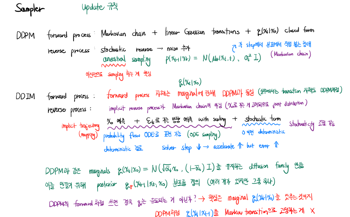
• DDPM: stochastic, many-step ancestral sampling
  • forward process: Markovian chain + linear Gaussian transitions + $q(x_t \mid x_0)$ closed-form
  • reverse process: stochastic — at each step, noise is sampled directly from the posterior distribution
  • $p_\theta(x_{t-1} \mid x_t) = \mathcal{N}(\mu_\theta(x_t, t), \sigma_\theta^2 I)$
  • core idea: discrete-time sampling
• DDIM: deterministic, fast
  • forward process: same marginals as DDPM, but the transition itself is not Markovian
  • reverse process: implicit (not a Markov chain) — considered as a joint distribution over $x_0$
  • reverse step: predict $\hat{x}_0$ + predict the direction toward $x_t$ (with scaling) + optional stochastic term
  • implicit trajectory: controllable stochasticity (η in the reverse step)
    • $\eta = 0$ → deterministic; can be mapped to a probability-flow ODE
  • deterministic path → solver step $N \downarrow$ accelerates but introduces discretization error

Solver

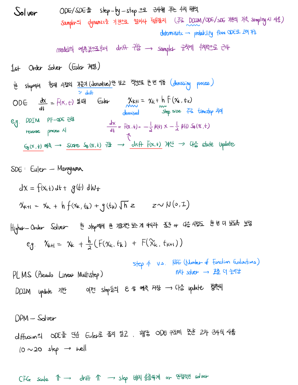
• diffusion sampling is solving an ODE / SDE step by step (numerical approximation)
• the sampler decides how much to integrate based on the model’s drift / score; the solver decides how each step is numerically computed

1st-order solvers (Euler family)

• one derivative per step, move along a straight line for one step
• for ODE $dx/dt = F(x, t)$: $x_{k+1} = x_k + h\, F(x_k, t_k)$
• DDIM is a PF-ODE-form Euler step: predict $\varepsilon_\theta(x_t, t)$ → score $s_\theta(x_t, t)$ → drift $F(x_t, t)$ → update $x_{t-1}$
• SDE Euler–Maruyama: $x_{k+1} = x_k + h\, f(x_k, t_k) + g(t_k)\sqrt{h}\, z, \; z \sim \mathcal{N}(0, \Sigma)$

Higher-order solvers

• evaluate the derivative at intermediate / next time points and average
  • e.g. Heun: $x_{k+1} = x_k + \tfrac{h}{2}\big(F(x_k, t_k) + F(x_{k+1}, t_{k+1})\big)$
• more accurate per step but increases the number of function evaluations (NFE)
• PLMS (Pseudo Linear Multistep): multi-step solver that reuses cached $\varepsilon$-predictions from previous steps → higher accuracy without extra NFE
• DPM-Solver: solver tailored to the diffusion ODE structure rather than treating it as a generic ODE → ~10–20 steps with good quality

Practical notes

• choice of solver determines the sample quality vs speed tradeoff
• with strong CFG / large drift, denser step placement near the high-drift region gives a more stable solver

ADM, Diffusion Likelihood & Efficient DiT

ADM (Diffusion Models Beat GANs)

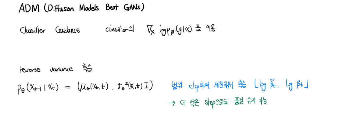
• Classifier Guidance: uses classifier’s $\nabla_x \log p_\phi(y \mid x)$ for conditioning
• reverse variance learned (rather than fixed)
  • $p_\theta(x_{t-1} \mid x_t) = \mathcal{N}(\mu_\theta(x_t, t), \sigma_\theta^2(x_t, t) I)$
  • log-variance clipped to a learned range $[\log \tilde{\beta}_t, \log \beta_t]$
• even fewer steps preserve quality

Diffusion Likelihood

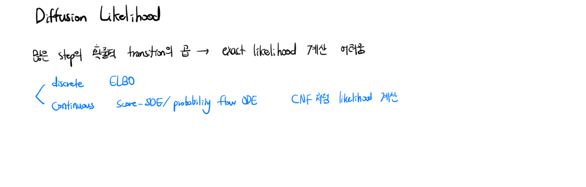
• many small stochastic transitions → exact likelihood is hard to compute
• discrete: ELBO
• continuous: Score-SDE / probability-flow ODE → CNF-style likelihood computation

Efficient DiT — Flash Attention & KV Cache

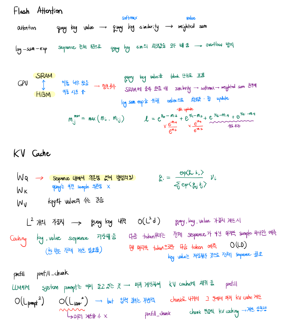
Flash Attention

• I/O-aware exact attention with tiled SRAM/HBM memory access
  • query · key → softmax-similarity → weighted sum
  • log-sum-exp trick: subtract max over entire sequence to avoid overflow
• SRAM tiling
  • load $Q, K, V$ in blocks into SRAM (fast on-chip memory)
  • GPU HBM ↔ SRAM data movement is the bottleneck → reduce round trips
  • compute similarity, softmax, and weighted sum on-chip in one pass
• online running max + log-sum-exp update
  • $m_i = \max(m_{i-1}, m_{i,j})$
  • $\ell_i = e^{m_{i-1} - m_i}\, \ell_{i-1} + e^{m_{i,j} - m_i}\, \ell_{i,j}$
  • update normalization stably as new blocks arrive

KV Cache

• weight matrices: $W_Q, W_K, W_V$ produce query/key/value at each token
  • query has no dependence on previous samples (within one decoding step)
  • key/value count grows with sequence length $L$
• compute cost per token: $O(L d^2)$
  • cached key/value tensors are stored once and reused across decoding steps
  • next token: only the last query needs to be computed against the full cached KV
• prefill vs decode
  • prefill: process the known prompt (system prompt etc.) once → fill the KV cache: $O(L_{\text{prompt}} d)$
  • decode: predict next token from cached KV → $O(L d)$ per step
• prefill chunk
  • split a large prompt into chunks
  • compute KV cache chunk-by-chunk to bound peak compute