• These notes were prepared while studying for technical interviews (e.g., Snap Inc., Krafton, etc.).
• Each entry contains a concise English summary, key math expressions, and excerpts from my original handwritten/typed study notes.

These notes cover the mechanics that make deep networks trainable: how gradients are computed, how parameters are updated efficiently, how to choose initial values, and how activations shape gradient flow.

Backpropagation

• efficiently compute gradients of a loss with respect to all parameters
  • based on the chain rule
  • enables training of deep neural networks via gradient-based optimization
• propagate error signals from the output layer backward through the network

Chain rule

• reusing intermediate derivatives → avoid redundant computations

Computation flow

• forward pass: compute activations and loss
• backward pass: compute gradients layer by layer from output to input
• each layer contributes a local derivative → gradients = products of local derivatives

Dynamic programming

• cache intermediate activations during the forward pass
• reuse activations during the backward pass to compute gradients efficiently
• complexity: linear in the number of parameters

Gradient Accumulation

• simulate a larger batch size by accumulating gradients over multiple forward/backward passes
  • delays parameter updates until enough gradients are accumulated
• useful for overcoming GPU memory limits

Gradient Checkpointing

• store only a subset of activations during the forward pass → saving memory
  • decompose the network into segments with checkpoints
• recompute the rest during backpropagation
  • reruns forward computation from the nearest checkpoint when needed
• trade additional computation for reduced memory usage

Optimizer

• update model parameters to minimize a loss function
• determine update direction and step size

Gradient Descent

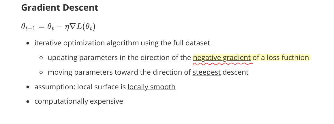
• iterative optimization algorithm using the full dataset
  • update parameters in the direction of the negative gradient of the loss function
  • moving parameters toward the direction of steepest descent
• assumption: local surface is locally smooth
• computationally expensive

Learning Rate

• hyperparameter $\eta$ controlling how aggressively parameters are updated

Step Size

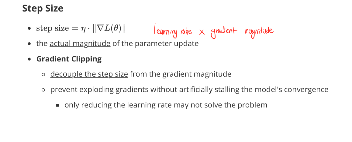
• step size $= \eta \cdot |\nabla \mathcal{L}(\theta)|$ (learning rate × gradient magnitude)
• the actual magnitude of the parameter update
• Gradient Clipping
  • decouple the step size from the gradient magnitude
  • prevent exploding gradients without artificially stalling convergence
    • only reducing the learning rate may not solve the problem

Stochastic Gradient Descent (SGD)

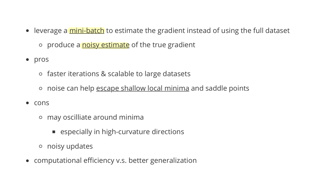
• leverage a mini-batch to estimate the gradient instead of using the full dataset
  • produce a noisy estimate of the true gradient
• pros
  • faster iterations & scalable to large datasets
  • noise can help escape shallow local minima and saddle points
• cons
  • may oscillate around minima
    • especially in high-curvature directions
  • noisy updates
• computational efficiency v.s. better generalization

Momentum

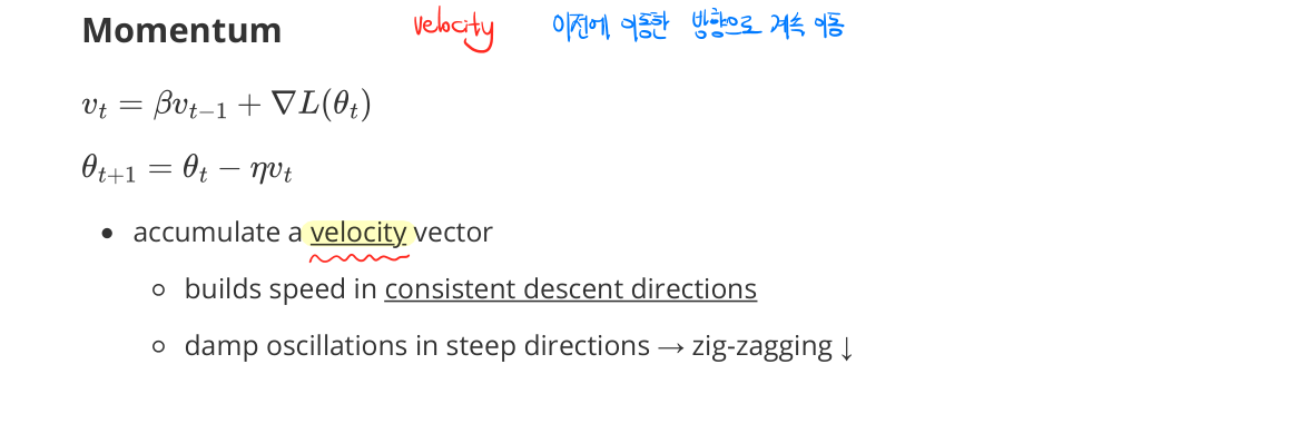
• accumulate a velocity vector
  • builds speed in consistent descent directions
  • damps oscillations in steep directions → zig-zagging ↓

RMSProp

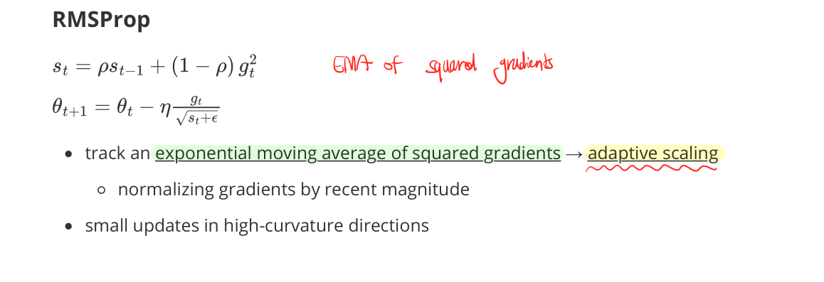
• track an exponential moving average of squared gradients → adaptive scaling
  • normalize gradients by recent magnitude
• small updates in high-curvature directions

Adam

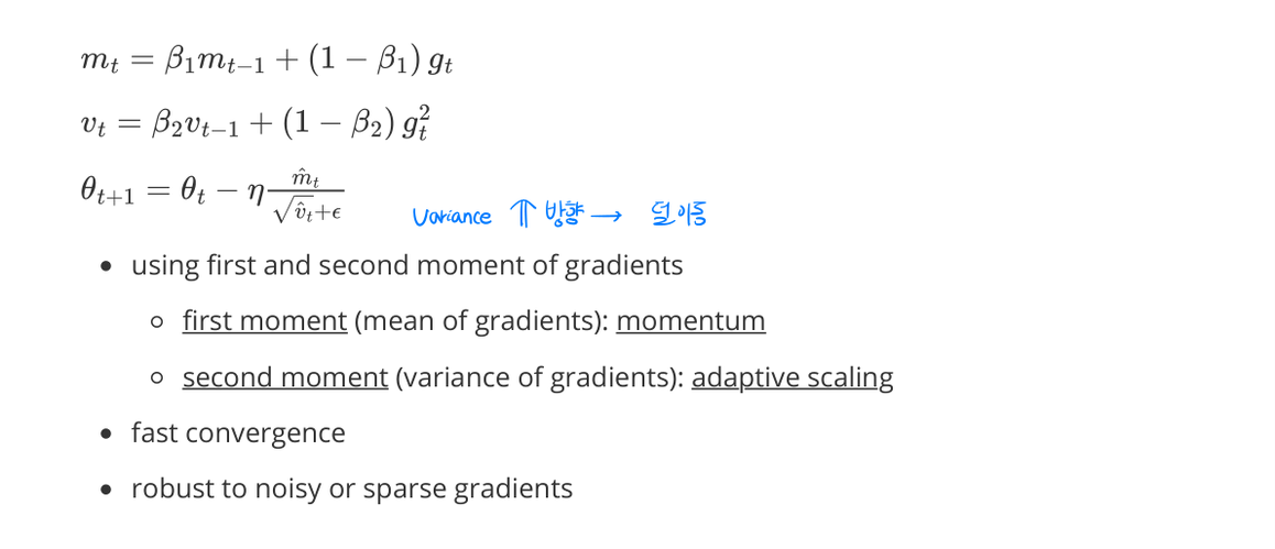
• using first and second moments of gradients
  • first moment (mean of gradients): momentum
  • second moment (variance of gradients): adaptive scaling
• fast convergence
• robust to noisy or sparse gradients

Activation Function

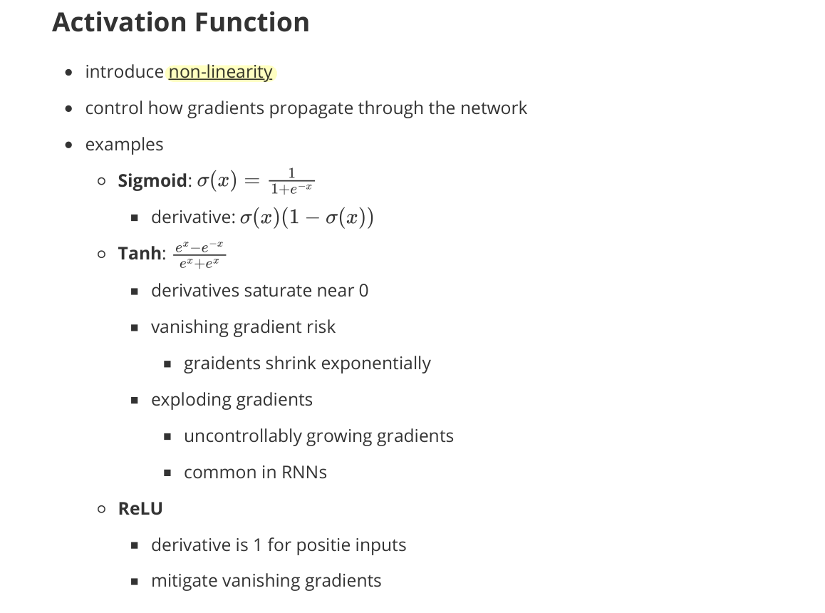
• introduce non-linearity
• control how gradients propagate through the network
• examples
  • Sigmoid: $\sigma(x) = \frac{1}{1 + e^{-x}}$
    • derivative: $\sigma(x)(1 - \sigma(x))$
  • Tanh: $\tanh(x) = \frac{e^x - e^{-x}}{e^x + e^{-x}}$
    • derivatives saturate near 0
    • vanishing gradient risk
      • gradients shrink exponentially
    • exploding gradients
      • uncontrollably growing gradients
      • common in RNNs
  • ReLU
    • derivative is 1 for positive inputs
    • mitigates vanishing gradients
    • example variants: Leaky ReLU, GELU

Initialization

• choosing initial values of model parameters before training
  • affects gradient flow and training stability
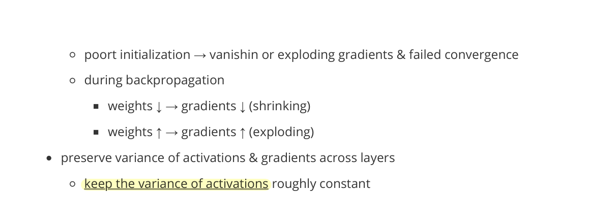
  • poor initialization → vanishing or exploding gradients & failed convergence
  • during backpropagation
    • weights ↓ → gradients ↓ (shrinking)
    • weights ↑ → gradients ↑ (exploding)
• preserve variance of activations and gradients across layers
  • keep the variance of activations roughly constant

Random Initialization

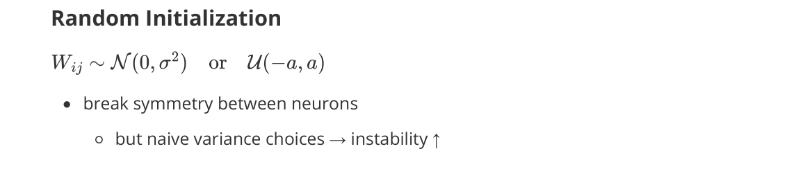
• break symmetry between neurons
  • but naive variance choices → instability ↑

Xavier Initialization

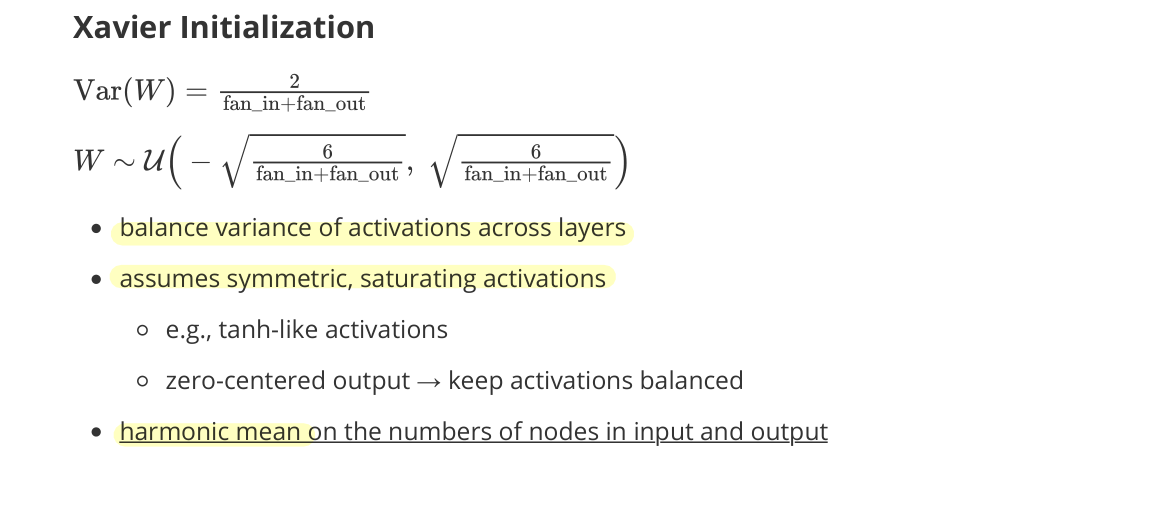
• balance variance of activations across layers
• assumes symmetric, saturating activations
  • e.g., tanh-like activations
  • zero-centered output → keep activations balanced
• harmonic mean on the numbers of nodes in input and output

He (Kaiming) Initialization

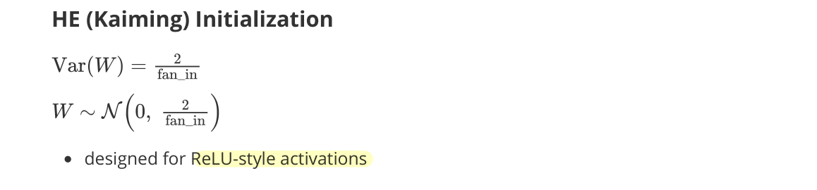
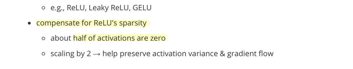
• designed for ReLU-style activations (e.g., ReLU, Leaky ReLU, GELU)
• compensate for ReLU’s sparsity
  • about half of activations are zero
  • scaling by 2 → preserve activation variance and gradient flow